Introduction
Over the course of the past few weeks, I’ve explored several different ways to model elections, with a focus on predicting the outcome of the upcoming 2020 presidential election. In this post, I’ll be making my final prediction before the election and discussing the choices I made when building my model. To make my prediction, I chose to use a two-sided ensemble model that predicts a separate vote share for the Democratic and Republican candidates, respectively. I considered both a pooled and an unpooled variation of the model, but ultimately decided to use the unpooled model to make my final prediction. Ultimately, my model predicts a somewhat narrow electoral college victory for Biden, with the candidate predicted to win 276 electoral votes to Trump’s 259 and flip key battleground states in the midwest (Michigan, Pennsylvania, Wisconsin, etc.) that broke for Trump in 2016 while falling short in several other swing states where the most recent polling has pointed to potential victories (Florida, Texas, Georgia, North Carolina).
Model Description
For the forecast, I used multiple linear regression to predict state-by-state vote shares for both the Democratic and Republican candidates as part of a weighted ensemble model. Each state’s party vote share prediction is comprised of two equally weighted predictions from two multiple linear regressions, with one using polling data to predict popular vote share (“polls”) and the other using lagged vote share, the change in the state’s white population, and whether the candidate’s party currently has incumbency status (“plus”). Here, the polling averages are fit into their own regression because the r-squared value tends to decrease when other covariates are added into the regression, so I thought it made the most sense to create a separate regression that could be fit with other predictive variables. While I initially tested a number of variables for the second regression, including economic variables such as Q2 gross domestic product (GDP) growth and Q2 real disposable income (RDI) growth alongside other demographic variables, such as the change in the 65+ population or the change in the Black population of a state, I ultimately found that my second regression generally yielded the highest r-squared values when it was fit with only the three variables I selected. Below, see what these regressions look like when written out as formulas:
y1 =β 0 + β 1 x lagged_voteshare + β 2 x white_change + β 3 x incumbent_party + ϵ
y2 = β 0 + β 1 x avg_poll + ϵ
y_prediction = (y1 x 0.5) + (y2 x 0.5)
Model Validation
When creating my model, I had initially experimented with both unpooled and pooled models in order to see which would be a better option for predicting 2020. With a completely unpooled model, each state’s prediction is made using only applicable historical data from that state, meaning that national trends are deemphasized and a certain critical mass of data is needed for each state in order to make a reliable prediction for each state’s vote share. Alternatively, a pooled model makes predictions for individual states based more heavily off of national trends and subsequently de-emphasizes state trends that can often be important for predicting particular state outcomes. Take a look at this summary table, which shows several metrics for in and out-of-sample fit for both the pooled and unpooled models I created:
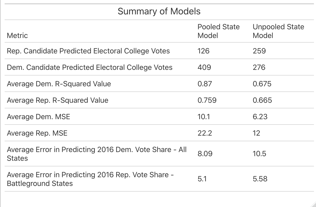
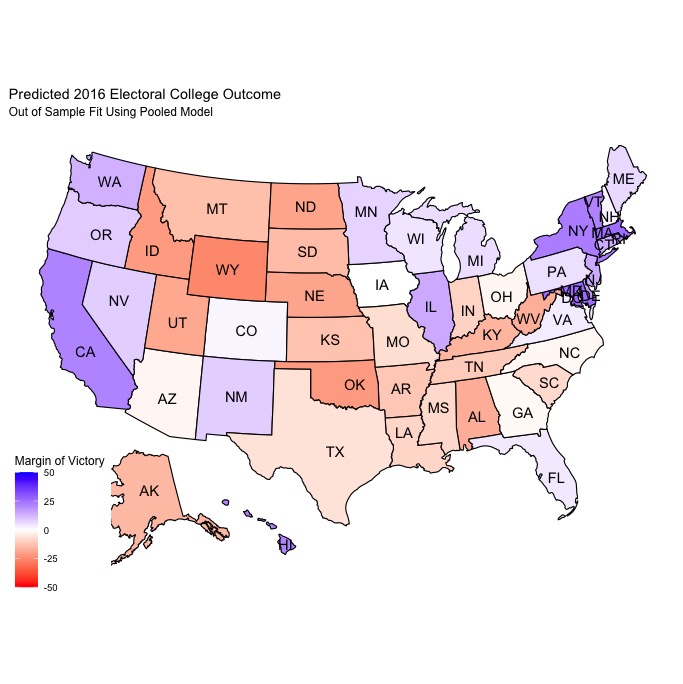
As you can see, both models have fairly high average R-squared values for both the Democratic and Republican sides of the model. The pooled model does have slightly higher average R-squared values overall, indicating that the proportion of the variance in the vote share that can be predicted from the predictive variables is greater than that of the unpooled model. However, the unpooled model ultimately had lower average mean squared error (MSE), meaning that the in-sample predictive performance was better than that of the pooled model. When both models were tested using leave-one-out validation to predict the results of the 2016 election, the pooled model generally performed better overall, but the unpooled model had less error when it came to predicting battleground states. Here are how both models predicted the 2016 election:
| Pooled | Unpooled |
|---|---|
 |
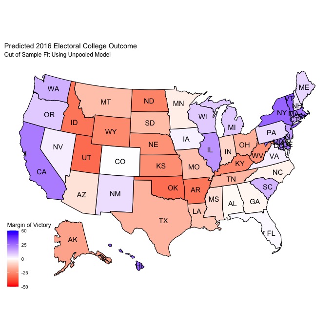 |
Both are pretty similar in terms of the electoral college predictions, with the pooled model predicting 2016 Democratic/Republican electoral college vote totals of 311/224 and the unpooled model predcting a 307/228 breakdown. These predictions (and the maps) are actually fairly similar to FiveThirtyEight’s predicted electoral college map and vote totals prior to the 2016 election.
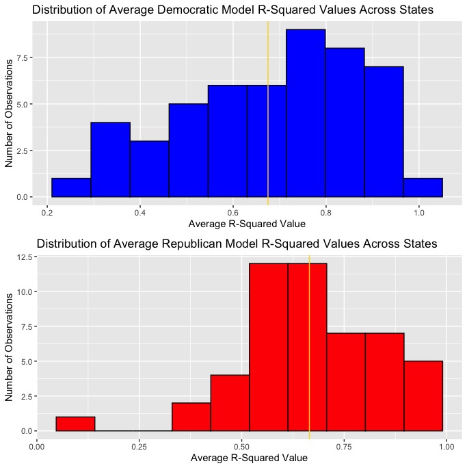
Ultimately, disproportionately lower MSE in the unpooled model in addition to its superior prediction power when it came to battleground states made it seem a little more plausible in terms of accurately predicting the 2020 election. These plots show the distribution of average R-squared and MSE values for the Democratic and Republican models across states.
| R-Squared | MSE |
|---|---|
 |
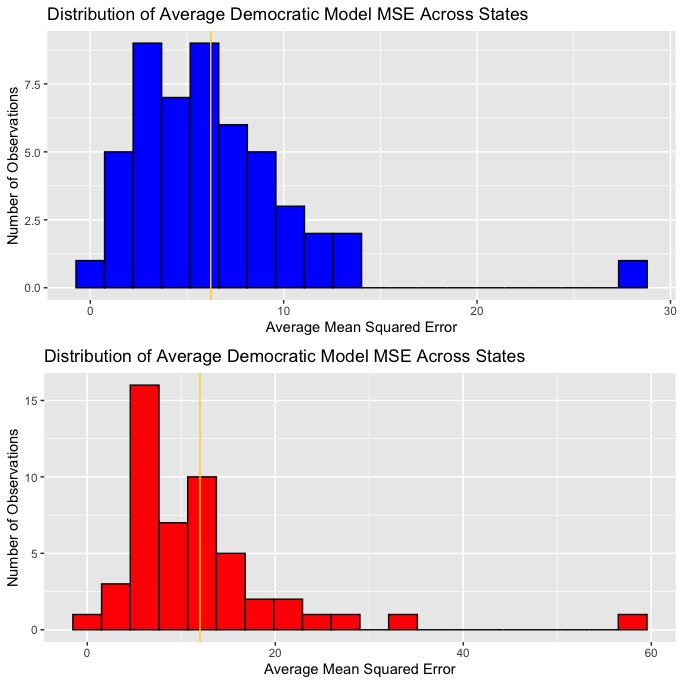 |
In all the plots, the average R-squared and MSE values are labeled with gold lines. As you can see, the Democratic regressions have both a higher average R-squared value and a lower average MSE, indicating that the Democratic vote share predictions should generally be somewhat more accurate than that of the Republican vote share predictions.
Prediction
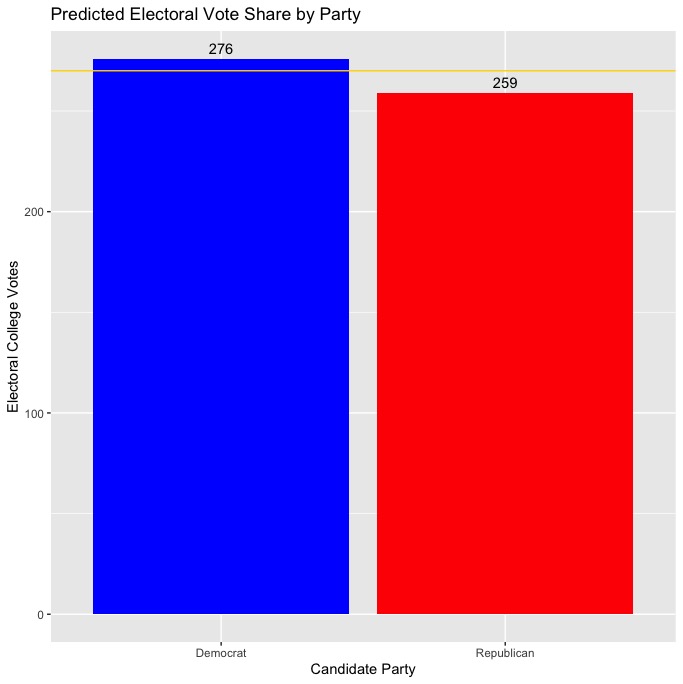
My model’s prediction for the candidate’s electoral college vote totals and the electoral college map is as shown below:
| Vote Totals | Map |
|---|---|
 |
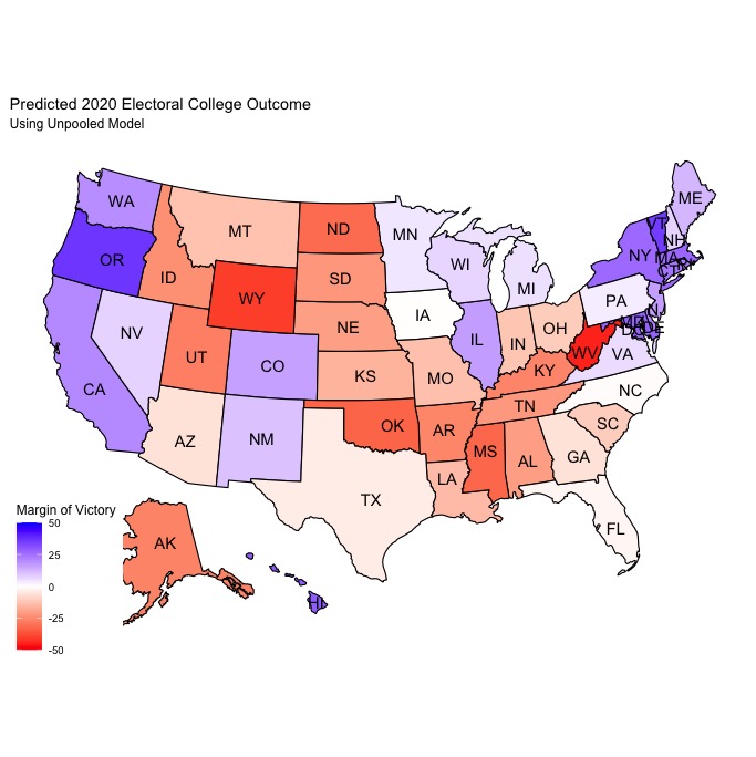 |
Ultimately, my model predicts that Biden will narrowly carry the electoral college with 276 electoral votes to Trump’s 259. This is certainly a more optimistic model for Trump than many professional models from forecasters like FiveThirtyEight and The Economist, but it still seemed to be a much more realistic prediction than that of the pooled model (which predicted a Biden landslide). Most traditionally “red” and “blue” states are predicted to vote the way you might expect, so the most interesting predictions are those for battleground/swing states as shown in the table below:
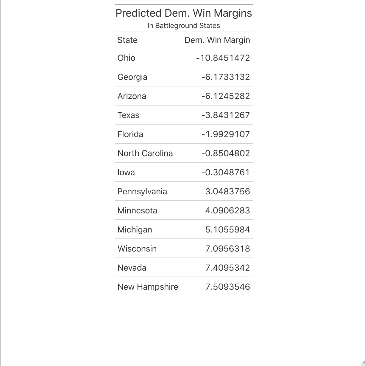
Ultimately, I think most of these predictions are fairly realistic. Reporting over the course of the past few days has shown Biden holding leads in Midwest states such as Michigan and Wisconsin while Trump gains ground in Arizona and North Carolina, so it makes sense that the model predicts comfortable victories in states like Wisconsin and Michigan. It isn’t shocking that the model predicts victories for Trump in traditionally red Sun Belt states like Texas, Arizona, and Georgia, but based on the latest polling from those states, it seems like the margins it predicts Biden to lose by are somewhat unrealistic. Considering that Biden leads in the most recent polling averages for Arizona and Georgia, and Trump is up by less than a point in Texas, it seems somewhat unlikely that Trump would be able to win each of these states by at least a 4-point margin. Based on the results of 2018 midterm elections in these states, where Democrats either narrowly won or lost Senate and Gubernatorial elections by margins of 3 points or less. I would say that these results are likely a consequence of choosing the unpooled model, which emphasizes trends in the state’s electoral history rather than national trends and thus leads to an overestimation of the GOP vote share in traditionally “red” states that have rapidly become competitive for Democrats in recent years. Still, the model seems to yield some very strong predictions for other swing states, such as North Carolina, Iowa, and Pennsylvania. North Carolina and Iowa are forecasted to break for Trump by less than a point each, which makes sense given Trump’s resurgence in the Iowa polls and the dominance of the GOP in modern North Carolina electoral history alongside polling averages that show Biden ahead by less than 3 points. It also seems highly likely that Pennsylvania will go for Biden by around 3 or so points, especially given that polling averages have him up by around 5 points over Trump. The most puzzling prediction my model yielded, however, is Ohio, which my model expects to go to Trump by a margin of around 10 points. I don’t think this is likely at all considering the most recent Ohio polling average shows only a 0.2 lead for Trump and his win margin in 2016 was less than 10 points. Still, due to the winner-take-all nature of each state’s electoral college votes (excluding the votes from Maine and Nebraska congressional districts) and the electoral college system, the margins of victory are largely inconsequential aside from their partisan disposition. While I think my prediction might end up being a little conservative in terms of underestimating the magnitude of a Biden victory as a result of focusing more narrowly on historical state electoral trends, I am more comfortable forecasting a close race in the wake of widespread overestimation of Clinton’s chances in 2016 than I am predicting a Biden landslide.
Uncertainty
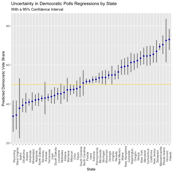
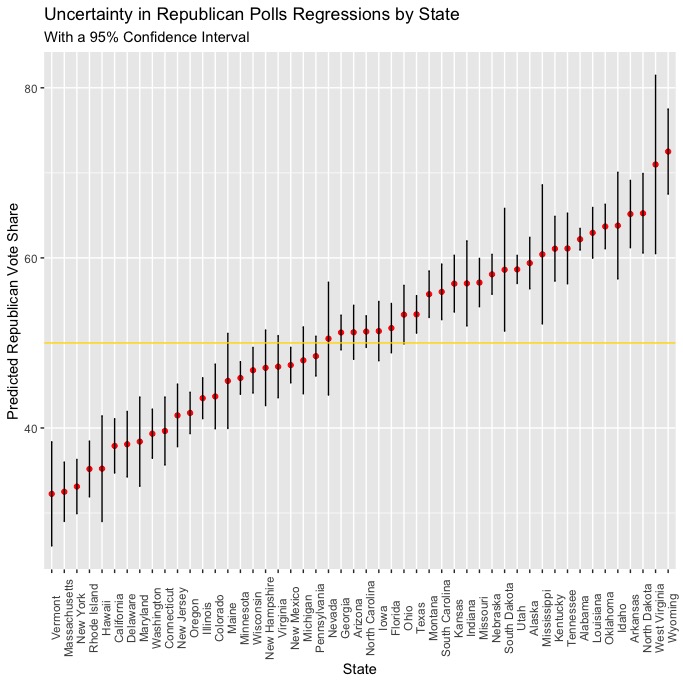
In order to visualize uncertainty, I created scatter plots with the points from both regressions (polls & plus) used to model each state’s Democratic and Republican vote shares, with vertical bars extending upward and downward to represent the lower and upper bounds of a 95% confidence interval, meaning that if we were to take 100 samples and find the 95% confidence interval for each of them, the real value would be within that range in 95 of the 100 samples. Let’s take a look at the confidence intervals from the polls & plus regressions:
Polls
| Democrat | Republican |
|---|---|
 |
 |
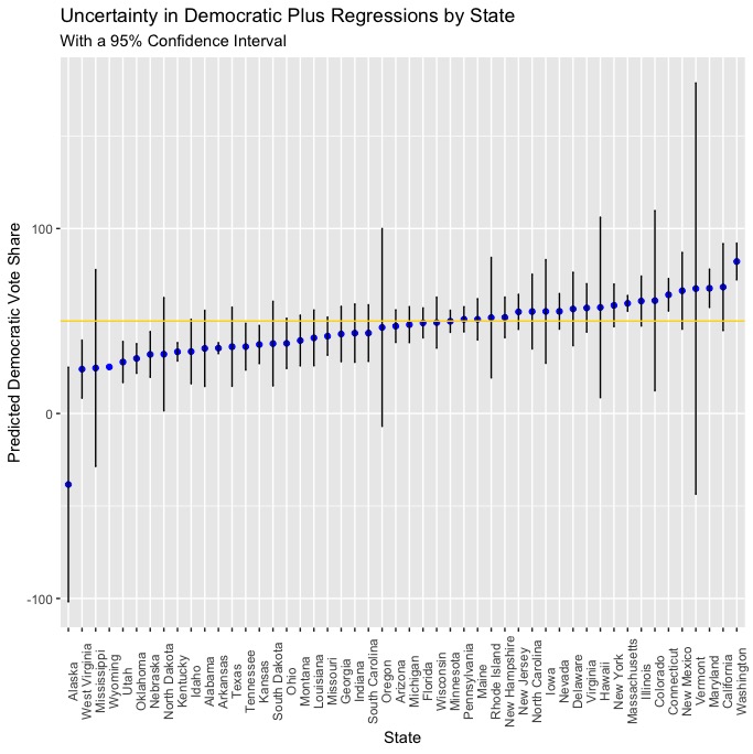
Plus
| Democrat | Republican |
|---|---|
 |
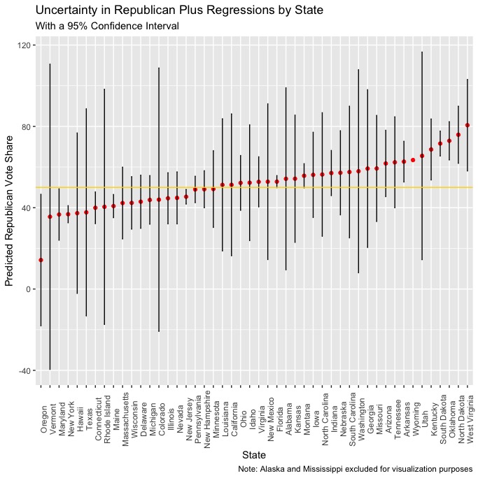 |
It seems as though there is much more uncertainty with the plus regressions than the polls regressions, which makes sense. The polls regressions are an incredibly simple model where polling averages are used to predict the respective Democratic and Republican vote shares, and we know that polls are generally one of the more predictive variables that can be used to model elections. The plus regressions are fit with more variables and have to incorporate all of them into a prediction, which would seem to explain why the confidence intervals are somewhat wider and the predictions are more uncertain. While including a variable like white_change is likely the best way to incorporate the changing demographics across the US into a model (at least in terms of thinking about how different demographic groups will impact the election), it will have a different level of predictive power in any given the historical trends in that state’s demographics (if any are apparent) and the current changes to that state’s demographics since 2016. Accounting for this uncertainty is partly why I chose to use an ensemble model, as the relatively higher certainty of the polls regressions can act to mitigate the magnitude of any errors that uncertainty from the plus regressions might be responsible for. It’s also notable that, on average, there is slightly more uncertainty in the predictions from the Republican polls and plus regressions.